How to compute mutational pressure

Without purifying selection

Say you have no purifying selection, meaning 0 infant mortality. All kids who are conceived grow up to be adults. But you have the following facts: every year after the age of 8, a male’s sperm cells accumulate on average 2 de novo mutations each. Also, you have the following chart (all the data in this article is simulated):

Where paternal age is the age of your father.

From just this knowledge we can compute the mutational pressure on the trait, which is how much the trait changes per generation due to the accumulation of new de novo mutations.

This is because mutational load correlates with paternal age.

This implies the following:

This is because the average mutational load given paternal age is just the line of best fit for the correlation between paternal age and mutational load. We know empirically that this line of best fit increases by two for every year of paternal age and has an intercept of 8.

What this means is we can just change the x axis of the first chart to be expected mutational load:

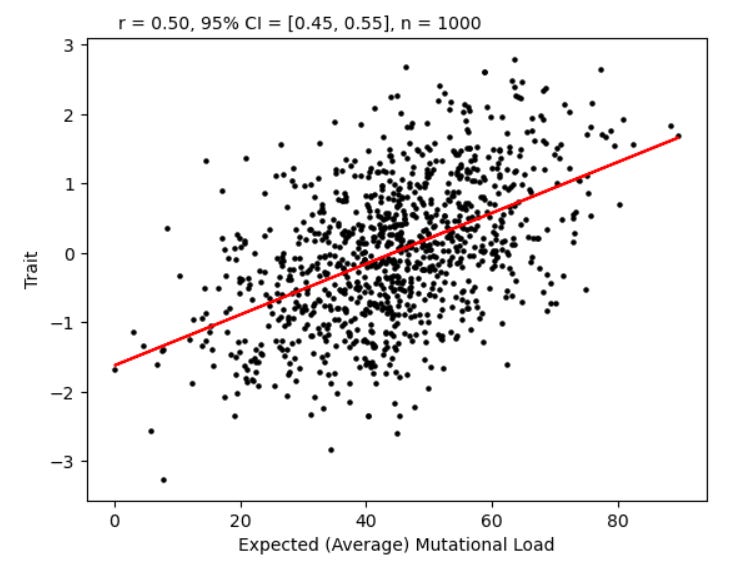
This chart shows the association between expected mutational load and the trait. If you look vertically, say at X=20, the average of all of those dots has mutational load 20. In turn, the average trait for those dots is given by the red line, it’s about -.85. Likewise, if you look at X=60, all the dots in a column above that marking sum up to have an average mutational load of 60. Their trait average is about 0.57.

So that line is Expected (Average) Trait = m(Average Mutational Load) + b:

\(E[T] = mE[M] + b\)

But it’s within a generation. Now we can predict how the trait will change due to mutation accumulation in the next generation.

\(\Delta E[T] = m\Delta E[M]\)

The intercept goes away because it cancels out in subtraction. Now we just solve for the change in mean mutational load. This is basically 2(E[Paternal age] - 8) because if the next generation is produced by fathers that average 30 years old, they will have average mutational load 2(30-8) = 44. So their load is 44 greater than the previous generation, or 1 SD. If we look back at the chart, they’ll have a 1.57 SD trait mean if you follow the line.

Now what is m? It’s a basic high school statistics formula the the slope of the line of best fit of the regression of x onto y is the following:

\(m = \frac{\sigma_y}{\sigma_x}r_{x,y}\)

Our SD(y) is 1 because the trait is standardized and we want the change in SDs. We can always standardize any trait we measure. r is the correlation between the trait and paternal age; this doesn’t change when you map paternal age onto expected mutational load, because r values are always the standardized line of best fit slope!

SD(x) is 2SD(paternal age) because x = expected value of mutational load = 2(Paternal Age) + c. We have measured the SD of paternal age to be 7 so SD(X) is 14.

Thus m = 0.5/14.

From this we get the formula above. The first term is the average mutation accumulation per generation and the second is just the correlation with the trait over the SD of expected mutational load.

Above is a 1 page summary of this article using mathematical argumentation.

There will be more in this series. We will add purifying selection into the model and compute the mutational pressure for leftism next. If you don’t want to miss out, make sure you subscribe: